Getting Started

Installing Python

pandapower is tested with up-to-date Python version, as listed at pypi. We recommend the Anaconda Distribution, which provides a Python distribution that already includes a lot of modules for scientific computing that are needed. Simply download and install the newest version of Anaconda and you are all set to run pandapower.

Of course it is also possible to use pandapower with other distributions besides Anaconda. It is however important that the following packages are included:

numpy
scipy
pandas
networkx
packaging
tqdm
deepdiff

Since some of these packages depend on C-libraries, they cannot be easily installed through pip on Windows systems. If you use a distribution that does not include one of these packages, you either have to build these libraries yourself or switch to a different distribution.

Installing pandapower

Through pip

The easiest way to install pandapower is through pip:

Open a command prompt (e.g. start–>cmd on windows systems)
Install pandapower by running:
```
 pip install pandapower[all]
```

Without internet connection

If you don’t have internet access on your system, pandapower can also be installed from local files:

Download and unzip the current pandapower distribution from PyPi under “Download files”.
Open a command prompt (e.g. Start-->cmd on Windows) and navigate to the folder that contains the pandapower code with the command cd <folder> :
```
cd %path_to_pandapower%\pandapower-x.x.x\
```
Install pandapower by running :
```
pip install -e .[all]
```

The option “-e” means that pip will provide an editable environment. In other words, the changes in the files in the directory with pandapower code will be considered. In case this is not necessary, an installation without the option -e will install the files in the environment as a copy, and the downloaded folder can be safely removed.

The option “all” means that not only the strictly required dependencies are installed, but also all the optional packages. Other options are: “docs”, “plotting”, “test”, “performance” (includes ortools for faster state estimation, numba and lightsim2grid that substantially improve the performance of power flow calculations), “fileio”, “converter”, “pgm” (includes the interface to power-grid-model as a power flow calculation engine). Most users can use the version “all” unless there are resons to avoid certain depemdencies.

Development Version

To install the latest development version of pandapower from github, simply follow these steps:

Download and install git.
Open a git shell and navigate to the directory where you want to keep your pandapower files.

Run the following git command:

 git clone https://github.com/e2nIEE/pandapower.git

Navigate inside the repository and check out the develop branch:
```
 cd pandapower
 git checkout develop
```
Open a command prompt (cmd or anaconda command prompt) and navigate to the folder where the pandapower files are located. Run:
```
 pip install -e .[all]
```
This registers your local pandapower installation with pip, the option -e ensures the edits in the files have a direct impact on the pandapower installation, and “all” installs all the optional dependencies.

Test your installation

A first basic way to test your installation is to import all pandapower submodules to see if all dependencies are available:

import pandapower
import pandapower.networks
import pandapower.topology
import pandapower.plotting
import pandapower.converter
import pandapower.estimation

If you want to be really sure that everything works fine, run the pandapower test suite:

Install pytest if it is not yet installed on your system:
```
pip install pytest
```

Run the pandapower test suite:

 import pandapower.test
 pandapower.test.run_all_tests()

If everything is installed correctly, all tests should pass or xfail (expected to fail).

A short introduction

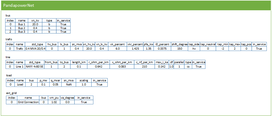
A network in pandapower is represented in a pandapowerNet object, which is a collection of pandas Dataframes. Each dataframe in a pandapowerNet contains the information about one pandapower element, such as line, load transformer etc.

We consider the following simple 3-bus example network as a minimal example:

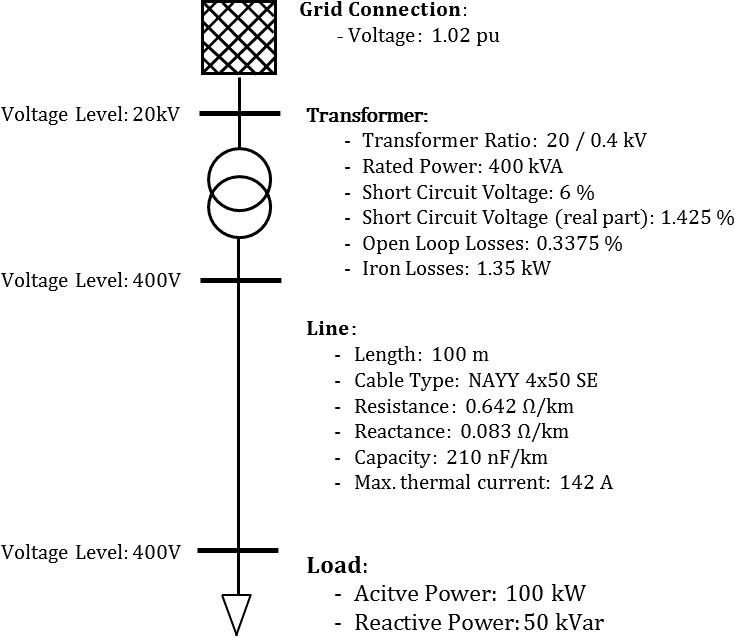
Creating a network

The above network can be created in pandapower as follows:

import pandapower as pp
# create empty net
net = pp.create_empty_network()

# create buses
b1 = pp.create_bus(net, vn_kv=20., name="Bus 1")
b2 = pp.create_bus(net, vn_kv=0.4, name="Bus 2")
b3 = pp.create_bus(net, vn_kv=0.4, name="Bus 3")

# create bus elements
pp.create_ext_grid(net, bus=b1, vm_pu=1.02, name="Grid Connection")
pp.create_load(net, bus=b3, p_mw=0.1, q_mvar=0.05, name="Load")

# create branch elements
pp.create_transformer(net, hv_bus=b1, lv_bus=b2, std_type="0.4 MVA 20/0.4 kV", name="Trafo")
pp.create_line(net, from_bus=b2, to_bus=b3, length_km=0.1, name="Line",std_type="NAYY 4x50 SE")

Note that you do not have to calculate any impedances or tap ratio for the equivalent circuit, this is handled internally by pandapower according to the pandapower transformer model. The standard type library allows comfortable creation of line and transformer elements.

The pandapower representation now looks like this:

Running a Power Flow

A powerflow can be carried out with the runpp function:

pp.runpp(net)

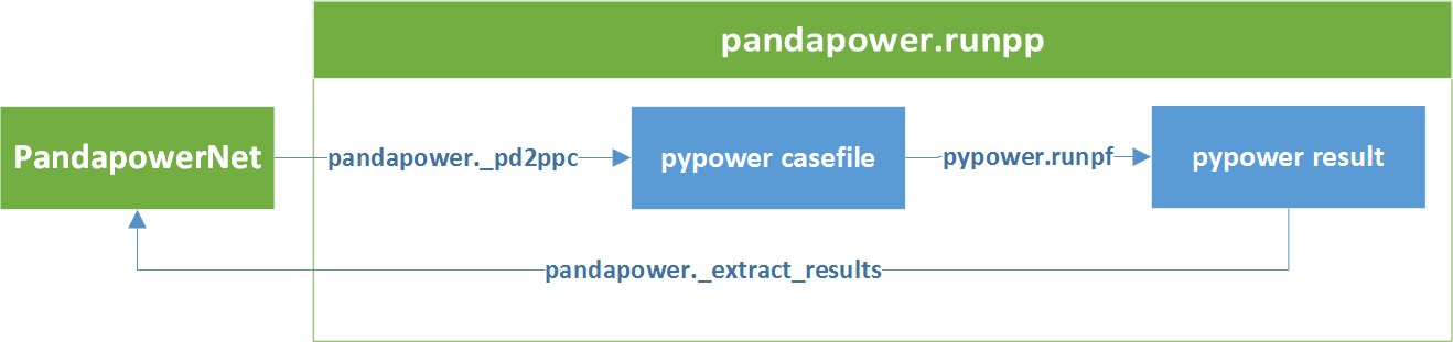
When a power flow is run, pandapower combines the information of all element tables into one pypower case file and uses pypower to run the power flow. The results are then processed and written back into pandapower:

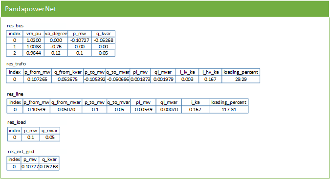
For the 3-bus example network, the result tables look like this:

All other pandapower elements and network analysis functionality (e.g. optimal power flow, state estimation or short-circuit calculation) is also fully integrated into the tabular pandapower datastructure.

This minimal example is also available as a jupyter notebook.

Interactive Tutorials

There are jupyter notebook tutorials on different functionalities of pandapower:

Basic introduction:

Data analysis and modelling error diagnostic:

Optimal power flow:

State estimation:

Configure and run a state estimation

Short-circuits:

Topology package:

Running topological graph searches

Plotting pandapower networks (static with matplotlib):

Plotting pandapower networks (interactive with plotly)

Time series calculation with the pandapower control module

YouTube Tutorials

You can also find some tutorials about the basics of pandapower on YouTube:

pandapower on YouTube